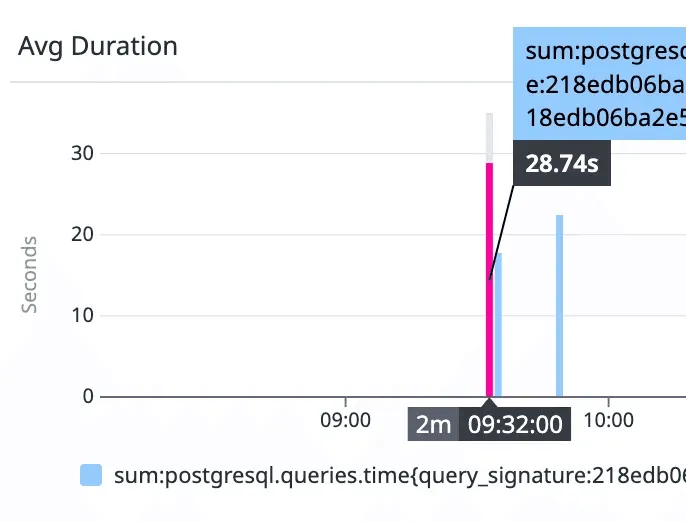
We recently shipped a new API endpoint at Mergify to surface metrics about newly introduced tests in a repository. The feature worked well during development, but once deployed to production, the endpoint started timing out. We expected a query to be nearly instant, but:

This is the story of what went wrong and how we fixed it.

The Feature

The endpoint returns tests that were first seen within a given time window, along with the pull request that introduced them. The data model involves three main tables:

• test_metrics, which stores test information, including a first_seen_sha column,

• pull_request_head_sha_history, which tracks which SHA belonged to which pull request over time,

• pull_request, containing the metadata we ultimately want to return.

The relationship between these tables is quite simple. Given a SHA from test_metrics, we need to find the pull request that had this SHA as its head at some point in its history.

The Naive Approach

Our first implementation followed what felt like a natural pattern. We built a subquery that maps every SHA to its corresponding pull request, then joined it with the test metrics:

WITH pr_for_sha AS (
  SELECT head_sha, ...
  FROM pull_request_head_sha_history 
  JOIN pull_request ON ...
  ORDER BY head_sha, timestamp DESC
)
SELECT * 
FROM test_metrics 
JOIN pr_for_sha ON pr_for_sha.head_sha = test_metrics.first_seen_sha 
WHERE

The intent reads clearly enough: build a lookup table mapping SHAs to pull requests, then use it to enrich the test metrics. The trouble is that PostgreSQL executes this query exactly as written, which turned out to be the root of our problem.

When we analyzed the query using EXPLAIN ANALYZE, the source of the slowdown became apparent:

Seq Scan on pull_request_head_sha_history (rows=660,958)
-> Hash Join with pull_request (rows=316,906)
-> Sort by (head_sha, timestamp DESC)
-> Unique

The database was dutifully scanning over 660,000 rows to construct a complete SHA-to-pull-request mapping for the entire system, only to then filter it down to match the handful of rows coming from test_metrics.

The filters on test_metrics were actually quite selective. Indeed, with the owner_id and time constraints in place, the table typically yielded somewhere between 10 and 50 rows. But those filters were being applied after the massive lookup table had already been built, which rather defeated the purpose.

What we had, in effect, was a join order problem. What we wanted was:

1. Filter test_metrics first, yielding roughly 50 rows,

2. For each of those rows, look up the corresponding pull request.

What we got instead was:

1. Build a mapping of all 660,000 SHAs to their pull requests,

2. Join the result with the 50 rows from test_metrics.

This is something like the "What is the "N+1 selects problem" in ORM (Object-Relational Mapping)?" in reverse, except here the "1" was a full table scan rather than a single query.

Enter LATERAL JOIN

A LATERAL join allows a subquery to reference columns from tables that appear earlier in the FROM clause. In practice, this means PostgreSQL will execute the subquery once for each row produced by the preceding table expression.

LATERAL joins tend to be particularly effective in a few specific scenarios: when you need the "first row per group" or "latest row per group" pattern using ORDER BY ... LIMIT 1; when the outer query is highly selective; and when you have proper indexes on the columns used in the correlation.

They are not universally superior, of course. If the outer query returns a large number of rows, you may simply be trading one full scan for many individual index lookups, which is not necessarily an improvement. But when the outer query is selective and the inner table is large, LATERAL joins can be remarkably effective.

We can now update our SQL query to use a LATERAL JOIN:

SELECT *
FROM test_metrics
JOIN LATERAL (
	SELECT ...
	FROM pull_request_head_sha_history
	JOIN pull_request ON ...
	WHERE head_sha = test_metrics.first_seen_sha  -- References the outer query.
	ORDER BY timestamp DESC
	LIMIT 1
) AS pr_for_sha
WHERE

The critical difference lies in the WHERE head_sha = test_metrics.first_seen_sha clause inside the subquery. This correlation fundamentally changes the execution strategy: PostgreSQL now applies the selective filters on test_metrics first, then performs a single index lookup for each resulting row rather than scanning the entire SHA history table upfront.

With an appropriate index on (head_sha, timestamp DESC), each of these lookups becomes an O(log n) operation instead of contributing to a full table scan.

The difference in complexity explains the dramatic performance gap:

┌──────────────┬──────────────────────────────────────────────────────┐
│   Approach   │                      Operations                      │
├──────────────┼──────────────────────────────────────────────────────┤
│ Subquery/CTE │ Scan 660K rows → Sort → Distinct → Join with 50 rows │
├──────────────┼──────────────────────────────────────────────────────┤
│ LATERAL      │ 50 rows × 1 index lookup each

The subquery approach scales with the total size of the SHA history table, regardless of how selective the outer query might be. The LATERAL approach, by contrast, scales with the number of test metrics actually returned, with each lookup benefiting from index access.

When you have 50 rows on one side and 660,000 on the other, the choice between these strategies matters quite a lot.

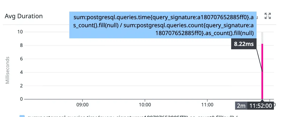
The data and the results remained identical. But, the execution path changed, yielding a three-order-of-magnitude improvement in response time.